The XSF format is internal
XCrySDen structure format. XSF
stands for
XCrySDen
Structure File. It is used to describe (i) molecular and
crystal structure, (ii) forces acting on constituent atoms, and
(iii) scalar fields (for example: charge density, electrostatic
potential). The main attributes of XSF format are:
- all records are in free format
- the XSF formatted file is composed from various sections
- each sections begins with the keyword
- there are two types of keywords: (i) single keywords,
and (ii) sandwich keywords, which are defined as:
- single keyword: section begins with a single keyword
and ends without an end-keyword
- sandwich keyword: section begins with a begin-keyword
(i.e.
BEGIN_keyword) and ends with an end-keyword
(i.e. END_keyword), where keyword is one
among keywords.
- all coordinates are in ANGSTROMS units
- all forces are in Hartree/ANGSTROM units
- the comment-lines start with the "#" character (see below)
The comment-lines were introduced to the XSF file starting from
XCrySDen version 1.4.
The comment-lines start with the
"#" character; comments are
allowed only between sections and not within a given section. Here
are two examples (correct and incorrect).
Correct example (comments are bewteen the sections):
 # this is a specification
 # of ZnS crystal structure

 CRYSTAL

 # these are primitive lattice vectors (in Angstroms)

 PRIMVEC
    2.7100000000    2.7100000000    0.0000000000
    2.7100000000    0.0000000000    2.7100000000
    0.0000000000    2.7100000000    2.7100000000

 # these are convetional lattice vectors (in Angstroms)

 CONVVEC
    5.4200000000    0.0000000000    0.0000000000
    0.0000000000    5.4200000000    0.0000000000
    0.0000000000    0.0000000000    5.4200000000

 # these are atomic coordinates in a primitive unit cell
 # (in Angstroms)

 PRIMCOORD
 2 1
 16      0.0000000000     0.0000000000     0.0000000000
 30      1.3550000000    -1.3550000000    -1.3550000000
|
Incorrect example (comment is within the section):
 ATOMS
  6    2.325243   -0.115261    0.031711
  1    2.344577   -0.363301    1.077589
#
# this is a comment on the wrong place
#
  6    0.007719   -0.041269    0.244204
  9    0.064656    1.154700    0.824420
  9   -0.042641   -0.911850    1.255074
  8   -1.071578   -0.152842   -0.539134
|
For MOLECULES the XSF format is very simple. The first line begins
with the
ATOMS keyword and then one specifies the
structural data for all atoms. An entry for an atom looks like:
AtNum X Y Z
where
AtNum stands for atomic number (or symbol),
while
X Y Z are Cartesian coordinates in ANGSTROMS
units. Here is one example:
 ATOMS
  6    2.325243   -0.115261    0.031711
  1    2.344577   -0.363301    1.077589
  9    3.131708   -0.909527   -0.638930
  9    2.736189    1.130568   -0.134093
  8    1.079338   -0.265162   -0.526351
  6    0.007719   -0.041269    0.244204
  9    0.064656    1.154700    0.824420
  9   -0.042641   -0.911850    1.255074
  8   -1.071578   -0.152842   -0.539134
  6   -2.310374    0.036537    0.022189
  1   -2.267004    0.230694    1.077874
  9   -2.890949    1.048938   -0.593940
  9   -3.029540   -1.046542   -0.203665
|
The XSF format allows to specify structures of different
periodicity. The keywords
MOLECULE,
POLYMER,
SLAB, and
CRYSTAL
designate the 0-, 1-, 2-, and 3-dimensional structures (i.e.
periodic dimensions are meant here). For crystal structures the
file begin with
CRYSTAL keyword. Then one needs to
specify the lattice vectors and the atoms belonging to the unit
cell.
XCrySDen accepts
two different setting of the unit cell. These are usually called
the primitive and the conventional unit cell. The corresponding
keywords are
PRIMVEC for primitive lattice vectors and
PRIMCOORD for atoms belonging to the primitive unit
cell. The
CONVVEC and
CONVCOORD have the
analogous meaning for the conventional unit cell.
Warning:
in XSF file the two settings of the unit cell are supposed to have
the same origin. If you want to specify some crystal structure with
two settings of the unit cell, that have different origins you will
have to create two XSF files. In practice only
PRIMVEC,
PRIMCOORD and
CONVVEC need to be specified, and then "conventional
coordinates" (
CONVCOORD) are generated by
XCrySDen itself, hence it is
never needed to specify the
CONVCOORD section
!!! Here is an example of ZnS crystal structure:
 CRYSTAL                                        see (1)
 PRIMVEC
    0.0000000    2.7100000    2.7100000         see (2)
    2.7100000    0.0000000    2.7100000
    2.7100000    2.7100000    0.0000000
 CONVVEC
    5.4200000    0.0000000    0.0000000         see (3)
    0.0000000    5.4200000    0.0000000
    0.0000000    0.0000000    5.4200000
 PRIMCOORD
 2 1                                            see (4)
 16      0.0000000     0.0000000     0.0000000  see (5)
 30      1.3550000    -1.3550000    -1.3550000
|
| Legend: |
| (1) |
this keyword specify the structure is
crystal
|
| (2) |
specification of PRIMVEC (in
ANGSTROMS) like:
ax, ay,
az
(first lattice vector)
bx, by,
bz
(second lattice vector)
cx, cy,
cz
(third lattice vector)
|
| (3) |
specification of CONVVEC (see
(2))
|
| (4) |
First number stands for number of atoms in the
primitive cell (2 in this case). The second number is always
1 for PRIMCOORD coordinates.
|
| (5) |
Specification of atoms in the primitive cell
(the same as for ATOMS section).
|
All that is needed to specify the forces acting on atoms is to
supplement the appropriate coordinate section (
ATOMS
or
PRIMCOORD). Now an entry for an atom would look
like:
AtNum X Y Z Fx Fy Fz
where
Fx Fy Fz stands for force components in X, Y and
Z direction, respectively. The force components are expressed in
Cartesian coordinate system in Hartree/ANGSTROM unit. Here is an
example of water molecule:
 ATOMS
  8   0.00000  0.00000  0.00000   -.05164  .00000 -.03999
  1   0.00000  0.00000  1.00000    .01769  .00000  .03049
  1   0.96814  0.00000 -0.25038    .03395  .00000  .00949
|
And here is an example for the periodic structure structure:
 SLAB
 PRIMVEC
   5.8859828533     0.0000000000     0.0000000000
   0.0000000000     5.8859828533     0.0000000000
   0.0000000000     0.0000000000     1.0000000000
 PRIMCOORD
 11 1
  6    3.674759   2.942992  -3.493103     -0.021668   0.000000  -0.057324
  1    4.121990   3.816734  -4.007689     -0.000478   0.001204   0.006657
  1    4.121990   2.069250  -4.007689     -0.000478  -0.001204   0.006657
  6    2.211226   2.942992  -3.493103      0.021668   0.000000  -0.057324
  1    1.763995   3.816734  -4.007689      0.000478   0.001204   0.006657
  1    1.763995   2.069250  -4.007689      0.000478  -0.001204   0.006657
  8    0.000000   0.000000  -2.719012      0.000000   0.000000  -0.050242
 47    4.448147   4.449892  -1.919011     -0.022812  -0.029123   0.007553
 47    4.448147   1.436093  -1.919011     -0.022812   0.029123   0.007553
 47    1.437838   4.449892  -1.919011      0.022812  -0.029123   0.007553
 47    1.437838   1.436093  -1.919011      0.022812   0.029123   0.007553
|
It is possible to specify several snapshots of a structure in the
XSF format. For example: the file can contain the data for all
structures that were created during an optimization run or
molecular-dynamics run. These structures can be displayed as
animation by
XCrySDen.
The main attributes of the animated XSF format are:
- the AXSF file begins with the
ANIMSTEPS
nstep
keyword, where nstep
stands for number of animation steps.
- number of atoms for all steps must be the same
!!!
- in fixed-cell animated XSF for crystal structures the unit cell
for all steps is taken to be the same
- in variable-cell animated XSF for crystal structures the unit
cell is specified for each animation step
- the
ATOMS and PRIMCOORD keywords are
prefixed by an integer number which is the sequential index of a
given snapshot. Therefore the syntax is ATOMS
istep and PRIMCOORD
istep.
- for variable-cell crystal structure the
PRIMVEC
and CONVVEC keywords are prefixed with sequential
index.
Here is an example of AXSF file. It shows different structures
during an optimization of water molecule. Note the index prefixes
after
ATOMS keywords.
 ANIMSTEPS 4
 ATOMS 1
  8    0.0000  0.0000  0.0000     -0.0516  0.0000 -0.0399
  1    0.0000  0.0000  1.0000      0.0176  0.0000  0.0304
  1    0.9681  0.0000 -0.2503      0.0339  0.0000  0.0094
 ATOMS 2
  8   -0.1480  0.0000 -0.1146      0.0020  0.0000  0.0015
  1   -0.0468  0.0000  0.9134     -0.0069  0.0000  0.0069
  1    0.8726  0.0000 -0.2740      0.0049  0.0000 -0.0084
 ATOMS 3
  8   -0.1032  0.0000 -0.0799      0.0013  0.0000  0.0010
  1   -0.0319  0.0000  0.9591      0.0011  0.0000 -0.0028
  1    0.9205  0.0000 -0.2710     -0.0025  0.0000  0.0018
 ATOMS 4
  8   -0.1102  0.0000 -0.0853      0.0001  0.0000  0.0000
  1   -0.0345  0.0000  0.9503     -0.0000  0.0000 -0.0000
  1    0.9114  0.0000 -0.2714     -0.0000  0.0000 -0.0000
|
Here is an example of animated XSF for the ZnS crystal structure
with the fixed unit-cell. Note the index prefixes after
PRIMCOORD keywords.
 ANIMSTEPS 2
 CRYSTAL
 PRIMVEC
    0.0000000    2.7100000    2.7100000
    2.7100000    0.0000000    2.7100000
    2.7100000    2.7100000    0.0000000
 PRIMCOORD 1
    2 1
    16      0.0000000     0.0000000     0.0000000
    30      1.3550000    -1.3550000    -1.3550000
 PRIMCOORD 2
    2 1
    16      0.0000000     0.0000000     0.0000000
    30      1.2550000    -1.2550000    -1.2550000
|
Here is an example of animated XSF for the ZnS crystal structure
with the variable unit-cell. Note the index prefixes after
PRIMVEC,
CONVVEC, and
PRIMCOORD keywords.
 ANIMSTEPS 2
 CRYSTAL
 PRIMVEC 1
    2.7100000    2.7100000    0.00000000
    2.7100000    0.0000000    2.71000000
    0.0000000    2.7100000    2.71000000
 CONVVEC 1
    5.4200000    0.0000000    0.00000000
    0.0000000    5.4200000    0.00000000
    0.0000000    0.0000000    5.42000000
 PRIMCOORD 1
    2 1
    16      0.0000000     0.0000000     0.00000000
    30      1.3550000    -1.3550000    -1.35500000
 PRIMVEC 2
    2.9810000    2.9810000    0.00000000
    2.9810000    0.0000000    2.98100000
    0.0000000    2.9810000    2.98100000
 CONVVEC 2
    5.9620000    0.0000000    0.00000000
    0.0000000    5.9620000    0.00000000
    0.0000000    0.0000000    5.96200000
 PRIMCOORD 2
    2 1
    16      0.0000000     0.0000000     0.00000000
    30      1.5905000    -1.5905000    -1.59050000
|
It is possible to specify one or several scalar fields (both 2D and
3D) as an
uniform mesh of values in the XSF formatted file.
The mesh can be
non-orthogonal. This scalar field meshes are
called
datagrids.
Datagrids in
XCrySDen
are general grids and not periodic one!!! What is meant by this
will be explained bellow. A general grid is a uniform grid that is
spanned inside some box, which is either non-orthogonal or
orthogonal. For a molecule such a box would be a bounding box,
while for crystal such a box would be a unit cell. However in a
grid that span a whole unit-cell some border points would be
redundant due to translational symmetry. Grids that omit these
redundant points are called periodic (by this convention a FFT
(fast-Fourier transform) mesh would be a periodic mesh). The
general vs. periodic grid concept is shown graphically here:
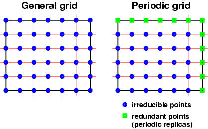
Note: datagrids in
XCrySDen are general grids !!!
The datagrid section is structured and organized in blocks. The
grids inside a block can be manipulated among themselves by
XCrySDen program. The
main attributes of XSF datagrids are:
| (1) |
the top datagrid section is called
BLOCK_DATAGRID and is sandwiched between
BEGIN_BLOCK_DATAGRID_xD and
END_BLOCK_DATAGRID_xD keywords, where x
stands for the dimensionality of the grid. Currently 2D and 3D
scalar grids are supported.
|
| (2) |
there can be an arbitrary number of
BLOCK_DATAGRID sections.
|
| (3) |
there can be an arbitrary number of datagrids
inside one BLOCK_DATAGRID section. All datagrids belonging to the
same BLOCK_DATAGRID must have the dimensionality as defined by
BEGIN_BLOCK_DATAGRID_xD keyword. These datagrids must
also share the following properties: (i) they should span the same
space (origin and the spanning vectors must be the same), and (ii)
they should have the same number of data-points. Each datagrid in a
BLOCK_DATAGRID is sandwiched inside
BEGIN_DATAGRID_xD_identifier and
END_DATAGRID_xD keywords, where x stands
for dimensionality of the grid and the identifier is
used as an identifier of the datagrid.
|
| (4) |
after the BEGIN_BLOCK_DATAGRID_xD
keyword and before the first DATAGRID_xD_identifier
keyword is a comment, which is used as an identifier for the
BLOCK_DATAGRID. It must be a single word!!!
|
| (5) |
the values inside a datagrid are specified in
column-major (i.e. FORTRAN) order. This means that values are
written as:
- C-syntax:
  for (k=0; k<nz; k++)
  for (j=0; j<ny; j++)
  for (i=0; i<nx; i++)
  printf("%f",value[i][j][k]);
- FORTRAN syntax:
  write(*,*)
  $  (((value(ix,iy,iz),ix=1,nx),iy=1,ny),iz=1,nz)
|
Above specifications may sound very fuzzy, hence let us clarify
this by looking at a very simple example. The
description of all records follows
after the example. Also take a look at
schematic presentation of the structure of
datagrids of below example.
l.01
l.02
l.03
l.04
l.05
l.06
l.07
l.08
l.09
l.10
l.11
l.12
l.13
l.14
l.15
l.16
l.17
l.18
l.19
l.20
l.21
l.22
l.23
l.24
l.25
l.26
l.27
l.28
l.29
l.30
l.31
l.32
l.33
l.34
l.35
l.36
l.37
l.38
l.39
l.40
l.41
l.42
l.43
l.44
l.45
l.46
l.47
l.48
l.49
l.50
l.51
l.52
l.53
l.54
l.55
l.56
l.57
l.58
l.59
l.60
l.61
l.62
l.63
l.64
l.65
|
 BEGIN_BLOCK_DATAGRID_2D
   my_first_example_of_2D_datagrid
   BEGIN_DATAGRID_2D_this_is_2Dgrid#1
     5  5
     0.0 0.0 0.0
     1.0 0.0 0.0
     0.0 1.0 0.0
       0.000  1.000  2.000  5.196  8.000
       1.000  1.414  2.236  5.292  8.062
       2.000  2.236  2.828  5.568  8.246
       3.000  3.162  3.606  6.000  8.544
       4.000  4.123  4.472  6.557  8.944
   END_DATAGRID_2D
   BEGIN_DATAGRID_2D_this_is_2Dgrid#2
     5  5
     0.0 0.0 0.0
     1.0 0.0 0.0
     0.0 1.0 0.0
       4.000  4.123  4.472  6.557  8.944
       3.000  3.162  3.606  6.000  8.544
       2.000  2.236  2.828  5.568  8.246
       1.000  1.414  2.236  5.292  8.062
       0.000  1.000  2.000  5.196  8.000
   END_DATAGRID_2D
 END_BLOCK_DATAGRID_2D

 BEGIN_BLOCK_DATAGRID_3D
   my_first_example_of_3D_datagrid
   BEGIN_DATAGRID_3D_this_is_3Dgrid#1
     5  5  5
     0.0 0.0 0.0
     1.0 0.0 0.0
     0.0 1.0 0.0
     0.0 0.0 1.0
       0.000  1.000  2.000  5.196  8.000
       1.000  1.414  2.236  5.292  8.062
       2.000  2.236  2.828  5.568  8.246
       3.000  3.162  3.606  6.000  8.544
       4.000  4.123  4.472  6.557  8.944

       1.000  1.414  2.236  5.292  8.062
       1.414  1.732  2.449  5.385  8.124
       2.236  2.449  3.000  5.657  8.307
       3.162  3.317  3.742  6.083  8.602
       4.123  4.243  4.583  6.633  9.000

       2.000  2.236  2.828  5.568  8.246
       2.236  2.449  3.000  5.657  8.307
       2.828  3.000  3.464  5.916  8.485
       3.606  3.742  4.123  6.325  8.775
       4.472  4.583  4.899  6.856  9.165

       3.000  3.162  3.606  6.000  8.544
       3.162  3.317  3.742  6.083  8.602
       3.606  3.742  4.123  6.325  8.775
       4.243  4.359  4.690  6.708  9.055
       5.000  5.099  5.385  7.211  9.434

       4.000  4.123  4.472  6.557  8.944
       4.123  4.243  4.583  6.633  9.000
       4.472  4.583  4.899  6.856  9.165
       5.000  5.099  5.385  7.211  9.434
       5.657  5.745  6.000  7.681  9.798
   END_DATAGRID_3D
 END_BLOCK_DATAGRID_3D
|
| Legend: |
| l.01 |
beginning of 2D block of
datagrids
|
| l.02 |
one word comment - used as an identifier for
this block
|
| l.03 |
beginning of the first 2D datagrid in a
block
|
| l.04 |
number of data-points in each direction (i.e.
nx ny for 2D grids)
|
| l.05 |
origin of the datagrid
|
| l.06 |
first spanning vector of the datagrid
|
| l.07 |
second spanning vector
|
| l.08-12 |
5x5 datagrid values in column-major mode
|
| l.13 |
end of the first 2D datagrid in a block
|
| l.14-24 |
these lines specify second 2D datagrid in a
block in totally analogous manner as the first 2D datagrid.
|
| l.25 |
end of 2D block of datagrids
|
| |
|
| l.27 |
beginning of 3D block of
datagrids
|
| l.28 |
one word comment - used as an identifier for
this block
|
| l.29 |
beginning of the first 3D datagrid in a
block
|
| l.30 |
number of data-points in each direction (i.e.
nx ny nz for 3D grids)
|
| l.31 |
origin of the datagrid
|
| l.32 |
first spanning vector of the datagrid
|
| l.33 |
second spanning vector
|
| l.34 |
third spanning vector
|
| l.35-63 |
5x5x5 datagrid values in column-major
mode
|
| l.64 |
end of the first 3D datagrid in a block
|
| l.65 |
end of 3D block of datagrids
|
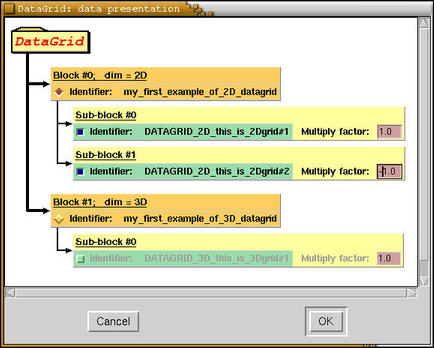
Here is a scheme of the structure of datagrids of above example as
displayed by
XCrySDen
program.
Bandgrids are variation on a theme of datagrids. They were
introduced for the visualization of Fermi surfaces and yields a
simplified format of
datagrids. Please notice that despite
their purpose they are still
general grids
and not periodic ones. The
bandgrid for the visualization
of Fermi surface should be defined as:
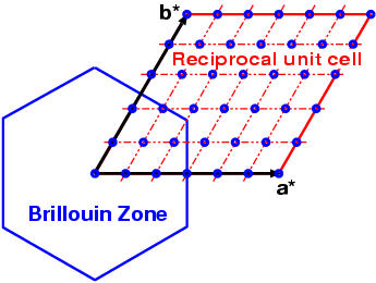
Please notice that the bandgrid span the reciprocal unit cell, not
the Brillouin zone !!! Points are later translated back to
Brillouin zone by
XCrySDen and Fermi surface is
rendered inside the Brillouin zone.
Warning: so far
XCrySDen uses
bandgrids solely for the visualization of Fermi surfaces
(the coresponding files are called BXSF, standing for Band-XSF). If
you want to render some other property as contours/isosurfaces you
must specify the scalar fields as
datagrids. This is
because the Fermi surfaces needs some special processing and
therefore bandgrids are automatically processed. The main
attributes of
bandgrids are:
| (1) |
the structure of bandgrids is similar
to datagrids
|
| (2) |
there can only be one BLOCK_BANDGRID
section
|
| (3) |
there can only be one BANDGRID in
BLOCK_BANDGRID
|
| (4) |
there can be an arbitrary number of
bands inside BANDGRID section, where BAND is ...
|
| (5) |
so far only 3D bandgrids are
supported
|
| BEWARE: |
the values inside a bandgrid are specified in
row-major (i.e. C) order. This
means that values are written as:
- C-syntax:
  for (i=0; i<nx; i++)
  for (j=0; j<ny; j++)
  for (k=0; k<nz; k++)
  printf("%f",value[i][j][k]);
- FORTRAN syntax:
  write(*,*)
  $  (((value(ix,iy,iz),iz=1,nz),iy=1,ny),ix=1,nx)
|
Here is a
bandgrid example. The description of the records
is below the example.
l.01
l.02
l.03
l.04
l.05
l.06
l.07
l.08
l.09
l.10
l.11
l.12
l.13
l.14
l.15
l.16
l.17
l.18
l.19
l.20
l.21
l.22
l.23
l.24
l.25
l.26
l.27
l.28
l.29
l.30
l.31
l.32
l.33
l.34
l.35
l.36
l.37
l.38
l.39
l.40
l.41
l.42
l.43
l.44
l.45
l.46
l.47
l.48
l.49
l.50
l.51
l.52
l.53
l.54
l.55
l.56
l.57
l.58
l.59
l.60
l.61
l.62
l.63
|
 BEGIN_INFO
   #
   # this is a sample Band-XCRYSDEN-Structure-File
   # aimed for Visualization of Fermi Surface
   #
   # Case:      just an example
   #
   # Launch as: xcrysden --bxsf example.bxsf
   #
   Fermi Energy: 0.83511
 END_INFO

 BEGIN_BLOCK_BANDGRID_3D
   here_we_have_some_examples
   BEGIN_BANDGRID_3D_simple_example
     2
     4 4 4
     0.0 0.0 0.0
     1.0 0.0 0.0
     0.0 1.0 0.0
     0.0 0.0 1.0
   BAND:  3
       0.000  0.192  0.385  0.577
       0.192  0.272  0.430  0.609
       0.385  0.430  0.544  0.694
       0.577  0.609  0.694  0.816

       0.192  0.272  0.430  0.609
       0.272  0.333  0.471  0.638
       0.430  0.471  0.577  0.720
       0.609  0.638  0.720  0.839

       0.385  0.430  0.544  0.694
       0.430  0.471  0.577  0.720
       0.544  0.577  0.667  0.793
       0.694  0.720  0.793  0.903

       0.577  0.609  0.694  0.816
       0.609  0.638  0.720  0.839
       0.694  0.720  0.793  0.903
       0.816  0.839  0.903  1.000
   BAND:  4
       1.000  0.942  0.885  0.827
       0.942  0.918  0.871  0.817
       0.885  0.871  0.837  0.792
       0.827  0.817  0.792  0.755

       0.942  0.918  0.871  0.817
       0.918  0.900  0.859  0.809
       0.871  0.859  0.827  0.784
       0.817  0.809  0.784  0.748

       0.885  0.871  0.837  0.792
       0.871  0.859  0.827  0.784
       0.837  0.827  0.800  0.762
       0.792  0.784  0.762  0.729

       0.827  0.817  0.792  0.755
       0.817  0.809  0.784  0.748
       0.792  0.784  0.762  0.729
       0.755  0.748  0.729  0.700
   END_BANDGRID_3D
 END_BLOCK_BANDGRID_3D
|
| Legend: |
| l.01 |
beginning of INFO section
|
| l.02-09 |
a hash "#" character stands for comment
|
| l.10 |
a "Fermi Energy:" string is a
marker for reading the value of Fermi energy
|
| l.11 |
end of INFO section
|
| |
|
| l.13 |
beginning of 3D block of
bandgrids
|
| l.14 |
one word comment - used as an identifier for
this block
|
| l.15 |
beginning of the 3D bandgrid
|
| l.16 |
number of bands in the bandgrid
|
| l.17 |
number of data-points in each direction (i.e.
nx ny nz for 3D grids)
|
| l.18 |
origin of the bandgrid
Warning: origin should be (0,0,0) (i.e. Gamma point)
|
| l.19 |
first spanning vector of the bandgrid (i.e.
first reciprocal lattice vector)
|
| l.20 |
second spanning vector
|
| l.21 |
third spanning vector
|
| l.22 |
beginning of the BAND with label 3
|
| l.23-41 |
4x4x4 values in row-major mode
|
| l.42 |
beginning of the BAND with label 4
|
| l.43-61 |
4x4x4 values in row-major mode
|
| l.62 |
end of the bandgrid
|
| l.63 |
end of 3D bandgrid block
|
![[Figure]](img/xcrysden-picture-small-new.jpg)