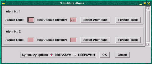
It is possible to use
XCrySDen as a tool when performing
the analysis of computed properties.
XCrySDen provides a subset of
options among all the options of the CRYSTAL
properties
program. This chapter is meant as a hand-on tutorial and we will go
trough all options that are available in
XCrySDen. First we should compute
some sample case (for examples one among the test cases that come
with standard CRYSTAL distributions). Then we do something
like:
              integrals < testCase.d12 > testCase.out
              scf > testCase.out
When the
testCase is finished successfully, among
other scratch files also the fortran unit 9 is produced (usually is
named as
fort.9 or
ftn9 depending on the
compiler). Then I usually do something like:
cp fort.9
testCase.f9
Now we can load this file into
XCrySDen. This can be achieved via
two ways:
| (1) |
via command line option, i.e: xcrysden
--crystal_f9 testCase.f9
|
| (2) |
specifying a filename of unit 9 via
File-->Open CRYSTAL-95/98/03/06 Properties
menu
|
After we load our unit 9 into
XCrySDen, the program displays the
structure and the
Properties menubutton gets activated. All
properties options of
XCrySDen are available under the
properties menubutton.
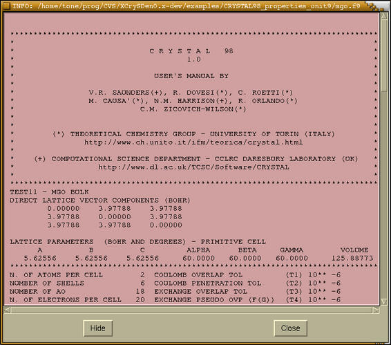
The first option in the
properties menu is the
Get INFO option. This option prints the
basic information about the case. After selecting this option the
program will ask whether we want the band widths to be included in
the basic info. If we answer positively, then the the following
window appears:
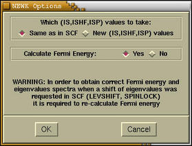
At the top of the
NEWK Options window we can enter new
NEWK values (refer to
CRYSTAL95/98 User Manual for the
explanation of the NEWK keyword). Below we can select whether we
want to recompute the Fermi energy. Answer according to your needs.
After pressing the
[OK] button a new window appears, which
holds a CRYSTAL output data.
This is a very useful option, which is accessible under the
Display Bandwidths menu.
First the
NEWK window pops-up, where one
can select new NEWK values (refer to
CRYSTAL95/98 User
Manual for the explanation of the NEWK keyword) and requests
for the recalculation of the Fermi energy. When we answer according
to our needs the following bar-graph window with band widths
appears:
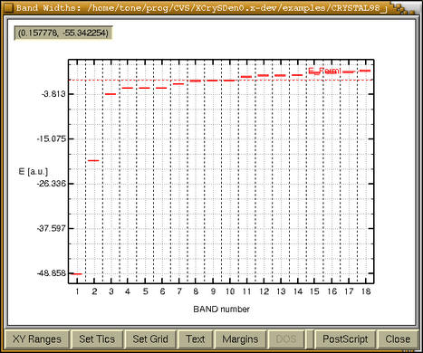
We immediately recognized that bands 1 and 2 are core states, bands
from 3 to 6 are semi-core states, bands from 7-10 are valence
bands, whereas bands from 11 on are unoccupied. Now we can refine
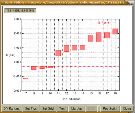
our plot pressing the
[XY Ranges] button and after playing a
while with other buttons, we get:
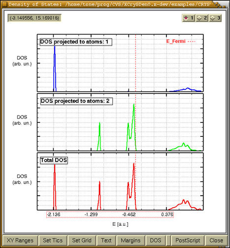
Density of States (DOS) can be calculated and displayed via
Density of States menu.
First the
NEWK window pops-up, where one
can select new NEWK values (refer to
CRYSTAL95/98 User
Manual for the explanation of the NEWK keyword) and requests
for the recalculation of the Fermi energy. When we answer according
to our needs a new window appears, where we specify the DOS
parameter:
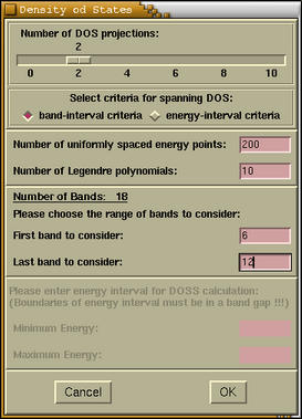
If we set the
number of DOS projections (NPRO) to zero
(default), then solely total DOS will be computed. For the
explanation of other parameters refer to
CRYSTAL95/98 User
Manual. When we input all parameters, then if the NPRO is zero
the total DOS and another window holding CRYSTAL output appear. On
the other hand, if the NPRO is greater then zero, then a new window
appears. Here we enter the projection parameters for each
projection.
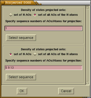
It is possible either to project the DOS to
set of some atomic
orbitals (AOs) or to
set of all AOs for some group of
atoms. This can be determining by choosing correct
radiobutton. If we select the first possibility then we should
enter the
ID numbers of appropriate AOs. In CRYSTAL AOs
are numbered in sequential fashion. To get an
ID number
for a particular AO we must know: (i) the order of atoms, (ii) the
basis set, and (iii) how the shell are ordered in CRYSTAL (the
order for
p type shell is:
x, y, z, while order
for
d type shell is:
2z2-x2-y2, xz, yz,
x2-y2, xy; refer to
CRYSTAL95/98
User Manual, p.50) Some information, such as number of AOs,
and sequential order of atoms can be obtained by reading the output
provided by
Properties-->Get
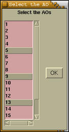
INFO menu option. If we press the
[Select
sequence] button, then a selection window appears. It merely
displays the ID numbers of either AOs or atoms (depending on the
prior choice of projection-type). Here we can select appropriate
numbers by holding down the
CTRL key and mouse-clicking.
When we are done then after pressing the
[OK] button the
projected DOS (only if it was specified) and total DOS appear. Also
another window holding the CRYSTAL output pops-up. Via
[XY
Ranges],
[Set Tics],
[Set Grid],
[Text],
[Margins] and
[Dos] buttons one can refine the plot
and make its appearance nicer. If one wants to change the font for
labels or width/color of curves one can simple double click these
items on the plot and a
configuration window will pop-up.
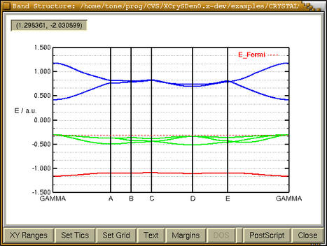
Band Structure (BAND) can be calculated and displayed via
Band Structure menu.
First the
NEWK window pops-up, where one
can select new NEWK values (refer to
CRYSTAL95/98 User
Manual for the explanation of the NEWK keyword) and requests
for the recalculation of the Fermi energy. When we answer according
to our needs a new window appears, where we select a k-path inside
Brillouin zone (BZ).
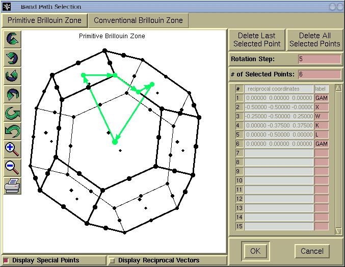
In above window we see two tabs entitled: (i)
Primitive
Brillouin Zone and (ii)
Conventional Brillouin zone.
The latter is provided only for informational purpose, namely, to
see the shape of the BZ tessellated according to the conventional
set of reciprocal vectors. Hence for real applications we stick to
Primitive Brillouin Zone and select a k-path by
mouse-clicking a special k-points. The BZ can be rotated by
holding-down left mouse button and dragging the mouse.
For a few Bravais lattice types, several common k-points will be
labelled automatically (thanks to Peter Blaha), such as GAMMA, X,
W, K, L points for the fcc lattice. The automatic k-point labbeling
currently supports the following Bravais lattice types:
- primitive cubic
- fcc
- bcc
- primitive tetragonal
- body centered tetragonal
- primitive orthorhomobic
When we are done with the k-points selection the [OK]
button should be pressed and a new window will appear.
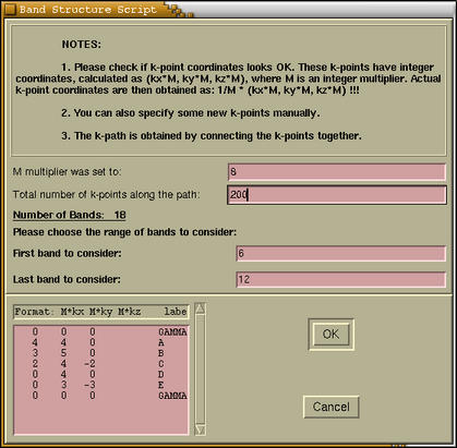
Here we specify the BAND parameters. Also we can enter some
additional k-points manually. After pressing the
[OK] button
the band structure is calculated and displayed.
Some properties like charge density and electrostatic potential can
be represented in 2D or 3D fashion, as contour plots or
isosurfaces.
XCrySDen
provides both kinds of plotting. Moreover for periodic structures
this plots have periodic attribute, meaning that the plots can be
replicated in periodic directions.
BEWARE: it is suggested
that only one 2D or 3D calculation is performed per
XCrySDen run. For example, rendering
first the charge density, and later on the electrostatic potentail
might result in Segmentation Fault. Instead, run the
XCrySDen twice. In first run render
the density, and in the second run the potential.
In order to produce an isosurface of some property (charge density,
electrostatic potential) proceed via
Properties-->Isosurfaces ... menu.
There one can choose among:
Charge
Density ,
Electrostatic
Potential and
Difference
Maps .
When we enter
Charge
Density or
Electrostatic
Potential option under the
Properties-->Isosurfaces ... menu, then
we first specify the grid parameters in the
3D
Map - Grid Specification window. In this window we find
several entries. Their meaning is the following:
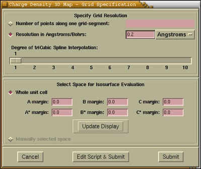
| [Grid Resolution] |
One can specify the resolution of the grid in
two ways: (i) by specifying the number of points along one grid
side ( n). Then the number of all points in the grid is on
the order of n3. At least for me this is not
very intuitive. (ii) by specifying the resolution in ANGSTROMS or
BOHRS. On the basis of my experiences the quality of rendered
isosurface can be classified according to the resolution as:
| Grid Resolution / ANGSTROMS |
Display of Isosurface |
| >0.3 |
poor |
| 0.3-0.15 |
medium |
| <0.15 |
good |
|
| [Interpolation] |
There is a possibility of interpolating a grid
by tri-cubic spline interpolation. At this stage I would suggest to
specify no interpolation (degree=1), as it will be possible to do
that later.
|
| [Space Selection] |
By default the space comprised by the whole
unit cell is selected for the CRYSTALS. For MOLECULES the space of
the bounding-box is selected instead. This box is just big enough
to hold the molecule. For SLABS and POLYMERS it is a "linear
combination" of both, namely, unit cell in the periodic directions
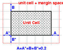
and bounding-box in the non-periodic directions. Then we have the possibility to specify the margins.
The margins are in fractional units (either with respect to unit
cell or bounding-box - depending on the periodicity of the
structure). Here is a simplified 2D example that explains the
meaning of this margins:
Important: Only after we press the [Update button]
the currently selected space will be rendered as transparent box.
On the figure below we see the unit-cell space selection with the
A=B=C=A*=B*=C*=0.2 margins.
|
There are three buttons on the bottom of
3D
Map - Grid Specification window. The function of these
buttons is the following:
| [Cancel] |
Cancels the process and closes the
window
|
| [Edit Script& Submit] |
User will be able to modify the input script
manually in an editor, just before it is submitted to calculation
with CRYSTAL properties module. Via this options it is
possible to alter the basis set, density matrix or some other
tuning. For example: ...insert example.... Editor is
chosen on the basis of EDITOR environmental variable. If this
variable does not exists, the vi editor is launched.
|
| [Submit] |
Submits the calculation to the CRYSTAL
properties module.
|
After CRYSTAL finishes calculating the 3D grid of points of
specified property the
Isosurface/Property-plane control
window appears, where we can control various parameters of
isosurface/property-plane rendering. The description of this window
and its parameters can be found
here.
When we enter the
Difference
Maps under the
Properties-->Isosurfaces ... menu, then
the following window pops-up:
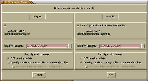
This window is divided in two parts:
Map A and
Map
B. Later on, the difference plots will be obtained by
subtracting the "Map B" from "Map A". For each map we should
specify a few parameters, such as: property to be calculated
(charge density, electrostatic potential) and some settings about
the density matrix. There is a possibility to load the unit 9 from
another file for the
Map B (the
[Load Crystal95's unit
9 from another file] checkbutton). For example if we want to
render the charge deformation density (i.e. charge density
difference between an SCF density and an atomic superposition
densities) then in both maps we select CHARGE DENSITY property and
an
[SCF density matrix] radiobutton for
Map A and
[Density matrix as superposition of atomic densities]
radiobutton for
Map B. Here it is not possible to specify
a new basis set for the atomic superposition density, but this will
be possible later on, where we will be able to edit the CRYSTAL
input script just before it is submitted to calculation. After
pressing the information the
3D Map - Grid
Specification window appear. Further information can be
read
here.
In order to produce a contour or color-plane plot of some property
(charge density, electrostatic potential) proceed via
Properties-->Properties on Plane
... cascade menu. There one can choose among:
Charge Density ,
Electrostatic Potential
and
Difference Maps .
When we enter
Charge
Density or
Electrostatic
Potential option under the
Properties-->Properties on Planes ...
menu, then we first specify the grid parameters in the
2D Map - Grid Specification window that is
shown below. The process is analogues to the
3D
grid specification, with the exception that here we select a 2D
region of space. The hints for specifying the grid resolution can
be found
here.
The second part (label
Select Plane for Property
Evaluation) of the
2D Map - Grid Specification window
is devoted to the selection of 2D region of space. We can do that
via two different procedures, which are chosen by pressing the
corresponding radiobutton, that is either
[Three-atoms spanning
parallelogram selection] or
[Atom centered selection].
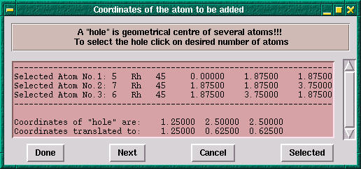
- [Three-atoms spanning parallelogram selection]
- After clicking this radiobutton a selection window pops-up. Here we select
three atoms that lie on the desired plane. Then we press the
[Selected] button on the selection window. After
that we press the [Update display] button on the 2D Map
- Grid Specification window the selected 2D region gets
rendered as transparent parallelogram. We can also specify the
margins AB, CD, AD, and BC. This margins are analogous to margins
A, A*, B, B*, C, C* margins for the
selection of 3D region. The updated margins will be rendered only
if we press the [Update display] button. We have also a
possibility to force the selected parallelogram to be rectangular.
This is achieved by pressing [Rectangular parallelogram]
checkbutton.
- [Atom centered selection]
- The Atom centered selection is a two-step procedure,
where we should select (1) an atom center and (2) a plane
direction. After clicking this radiobutton the following window
appears:
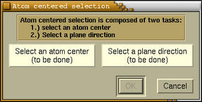
On this window two buttons named [Select an atom center] and
[Select a plane direction] stand for the two tasks that
should be done. At the bottom of these buttons is either a "(to be
done)" or "(done)" label. These remind us on the state of each
task, namely, is the task already done or yet to be done. The
selection window will pop-up when either
one of these buttons is pressed. When pressing the [Select an
atom center] button we should select one atom and press the
[Selected] button on selection
window. On the other hand when pressing the [Select a plane
direction] we should select three atoms that define desired
plane and press the [Selected] button on the selection window. When both tasks are completed we
should press the [OK] button on the Atom centered
selection window. Then we can press the [Update
Display] button on the selection
window to render the selected 2D region.
Three button are located at the bottom of
2D
Map - Grid Specification window. The description of their
function can be found
here.
The process of creating
2D Difference Maps is analogous to
the creation of
3D Difference Maps. First
we specify the
difference map
parameters and then we select the
2D region of
space, where the 2D difference map will be calculated.

![[Figure]](img/xcrysden-picture-small-new.jpg)